Dynamic SBI for cosmological field-level inference

Oleg Savchenko

o.savchenko@uva.nl

Perimeter Institute for Theoretical Physics, 8th June 2026

Work with:

Christoph Weniger

Guillermo Franco Abellán

Florian List

Noemi Anau Montel

Pieter Oehlers

Yannick Wischaupt

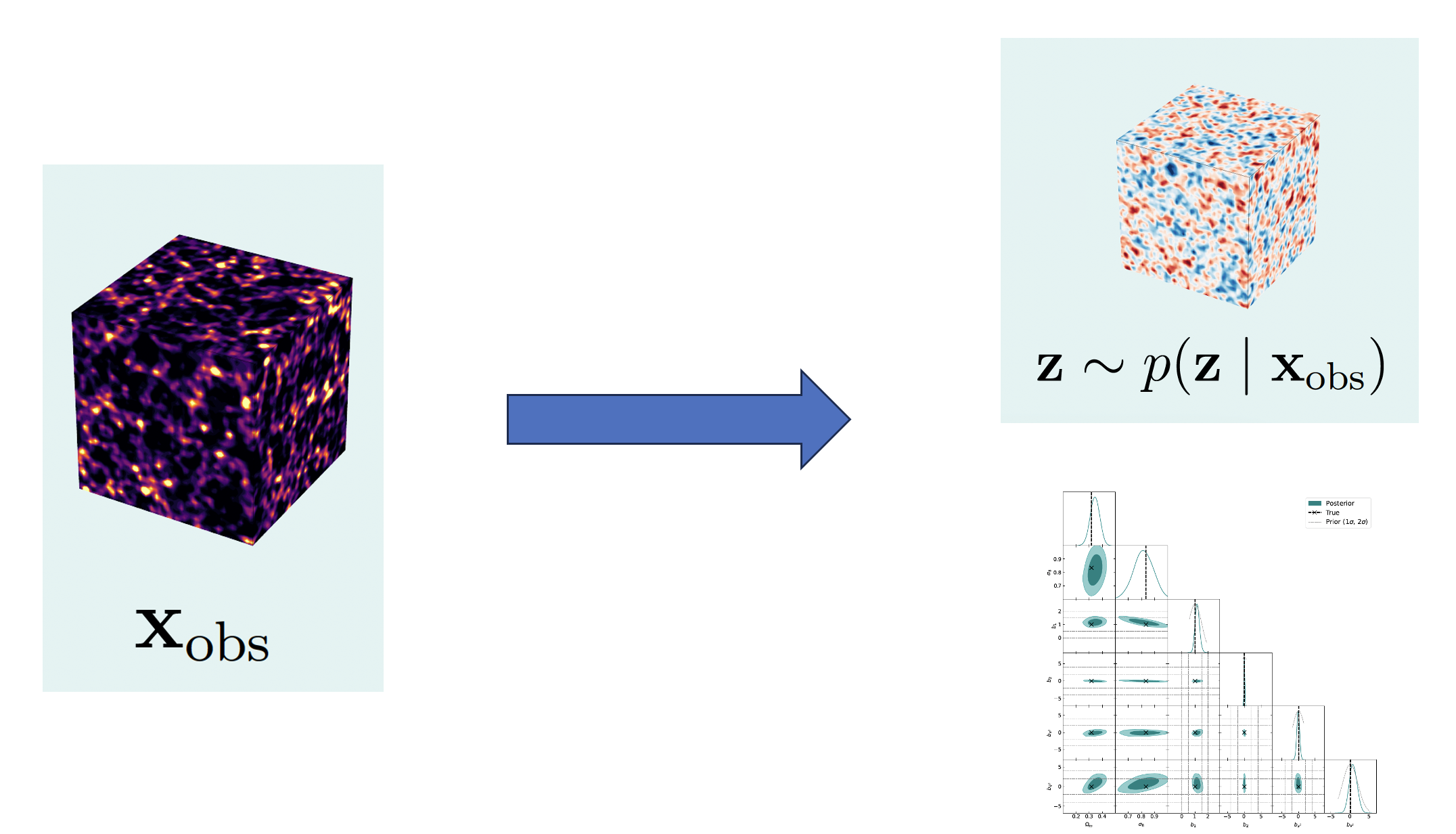
Field-level inference

Reconstructing a physical field allows to extract the maximal amount of information

\[ p(\mathbf{z}_{\mathrm{IC}}, \boldsymbol{\theta}|\mathbf{x}_{\mathrm{obs}}) = \;? \]

Review: Leclercq, 2509.13435

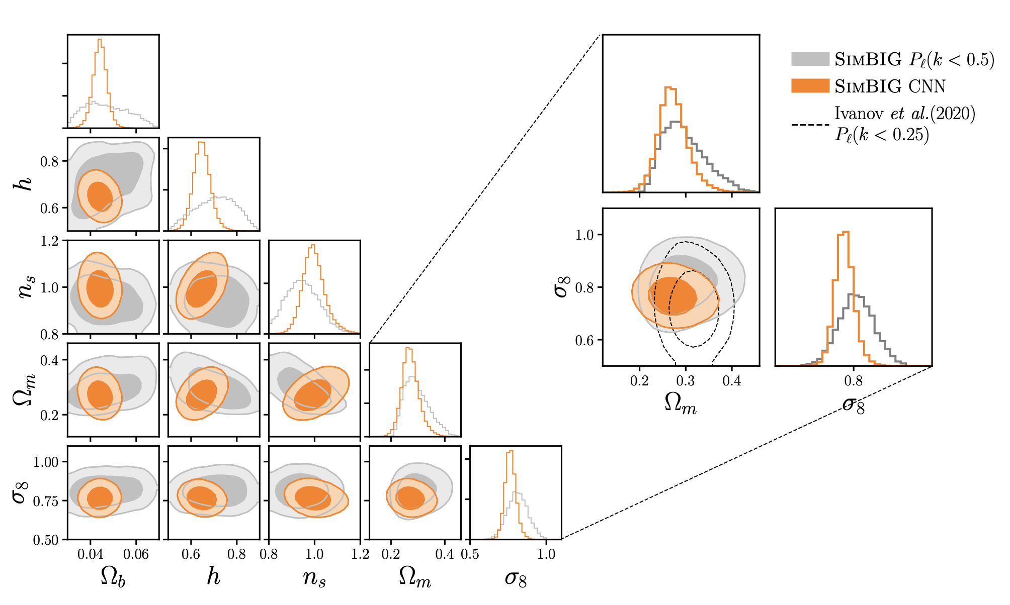
Optimal parameter constraints

The full field contains substantially more information than low-dimensional summaries such as the power spectrum!

\[ \langle \delta_{\mathrm{m}}(\mathbf{k})\,\delta_{\mathrm{m}}(\mathbf{k}')\rangle = (2\pi)^3\,\delta^3_{\mathrm{D}}(\mathbf{k}+\mathbf{k}')\,P_{\mathrm{mm}}(k) \]

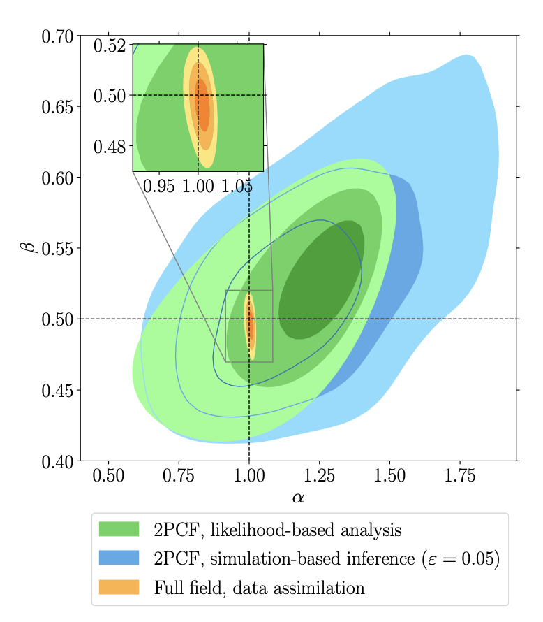
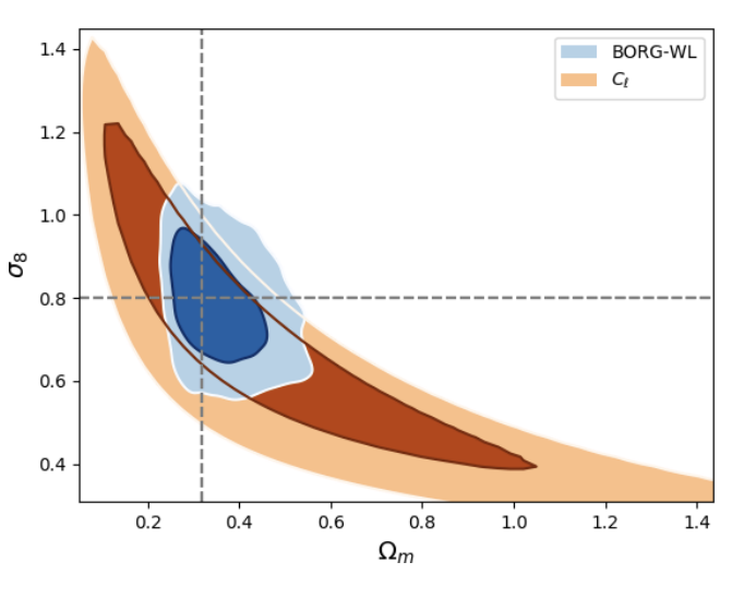
Leclercq+, 2103.04158

Porqueres+, 2108.04825

Lemos+, 2310.15256

Reconstructing fields

Porqueres+, 2304.04785

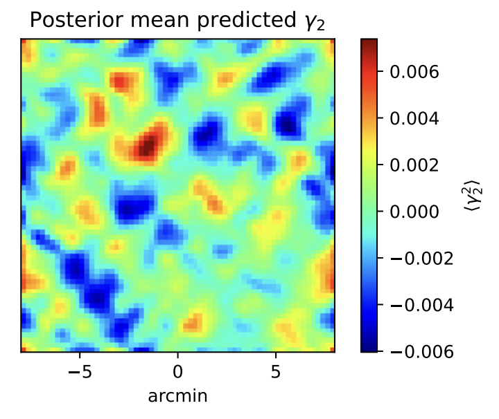
Weak lensing shear

Elbers+, 2307.03191

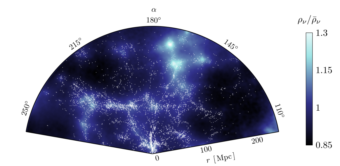
Neutrino field

Jasche+, 1806.11117

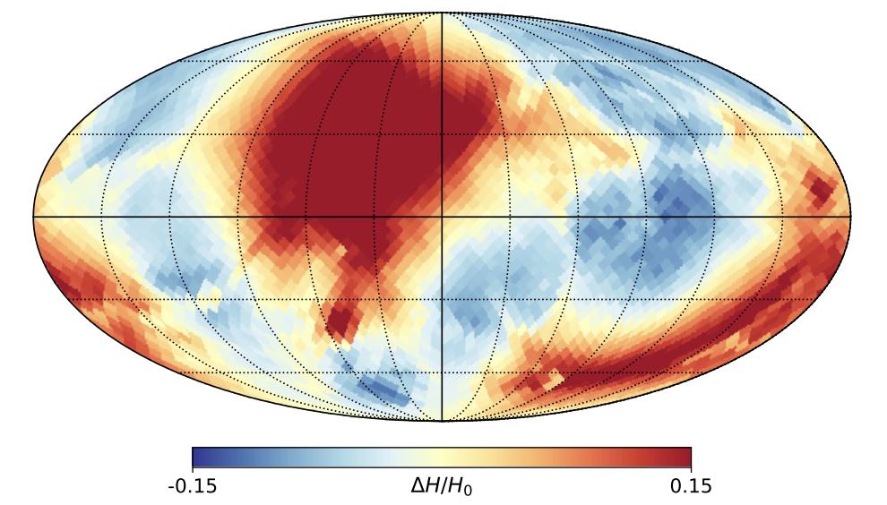
Hubble parameter uncertainties

Hutschenreuter+, 1803.02629

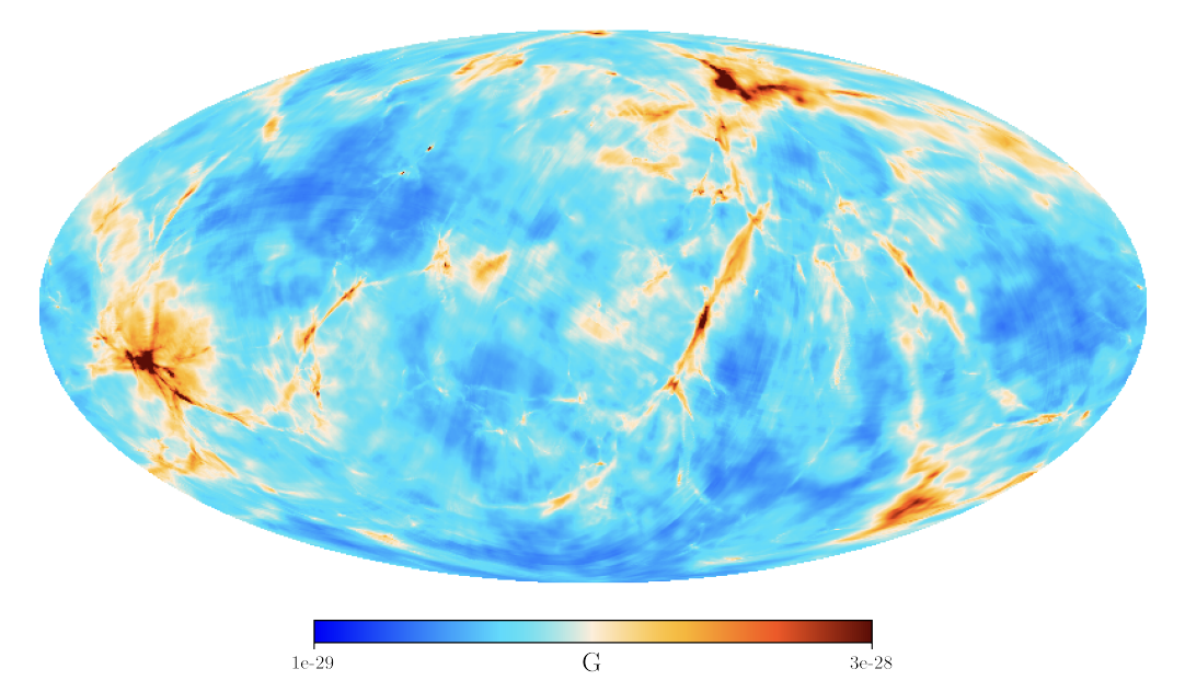
Magnetic field

Mass estimation and evolution

history, velocity fields, BAO,

\(f_{\text{nl}}\), 21 cm, weak lensing...

Simulation-based inference (SBI)

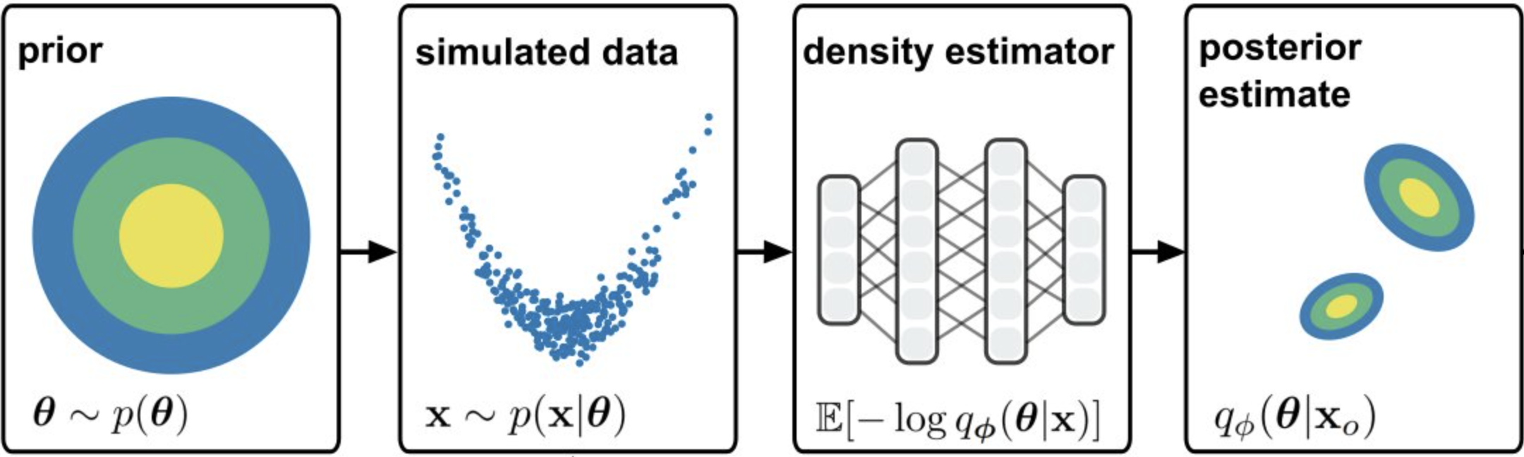
Unknown likelihood on nonlinear scales:
for small-scale cosmological observables, the likelihood \(p(\mathbf{x} \mid \boldsymbol{\theta})\) is not analytically tractable.

See reviews:

Cranmer+, 1911.01429
Deistler+, 2508.12939
Weniger, TASI lectures

Picture credit: Deistler+, 2210.04815

https://simulation-based-inference.org/

https://sbi.readthedocs.io/

\[ \underbrace{p(\boldsymbol{\theta}|\boldsymbol{x})}_{\textcolor{#8B6FC4}{\mathrm{posterior}}} = \frac{\overbrace{p(\boldsymbol{x}|\boldsymbol{\theta})}^{\textcolor{#D4783A}{\mathrm{likelihood}}}}{\underbrace{p(\boldsymbol{x})}_{\textcolor{#5A9E6A}{\mathrm{evidence}}}}\,\underbrace{p(\boldsymbol{\theta})}_{\textcolor{#C05858}{\mathrm{prior}}} \]

Neural Posterior Estimation (NPE)
Neural Likelihood Estimation (NLE)
Neural Ratio Estimation (NRE)

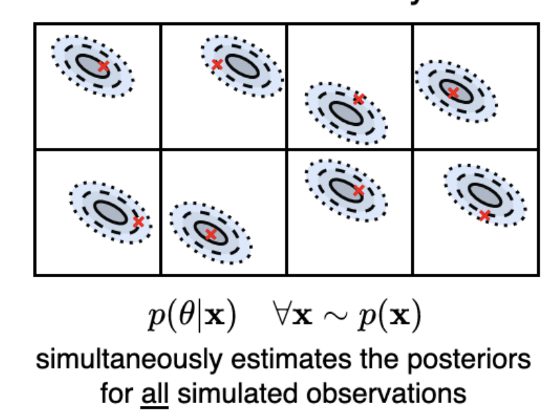
Amortized vs adaptive SBI

Amortized

Train once, then infer many times
High upfront simulation/training cost
Reusable for many \(\mathbf{x}_{\mathrm{obs}}\)
Learns a global inference network
Harder to converge to precise posteriors

Adaptive

Adaptively update the proposal and training set
Better precision/convergence
Targeted to one observation
Focuses simulations on relevant regions
Often more sample-efficient for one target

Cole+, 2111.08030

Round 1

→

Round 2

→

…

→

Round 6

Animation credit: N. Anau Montel

Adaptive inference in `Falcon`

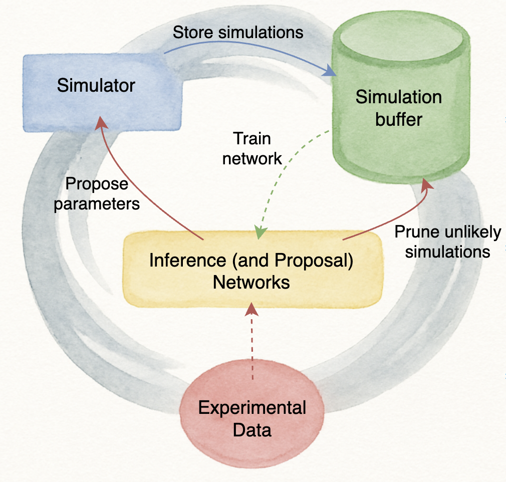
Framework for asynchronous distributed computing on multiple nodes
Training set evolves during training for adaptive inference: new samples are drawn from the proposal distribution
Some nodes simulate, some nodes train to do inference

cweniger/falcon
Lyu+, https://arxiv.org/abs/2510.13997

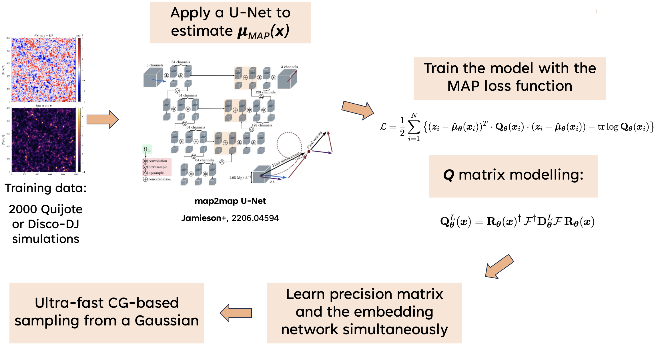
Gaussian NPE

OS+, 2410.15808, 2502.03139

GNPE Inference

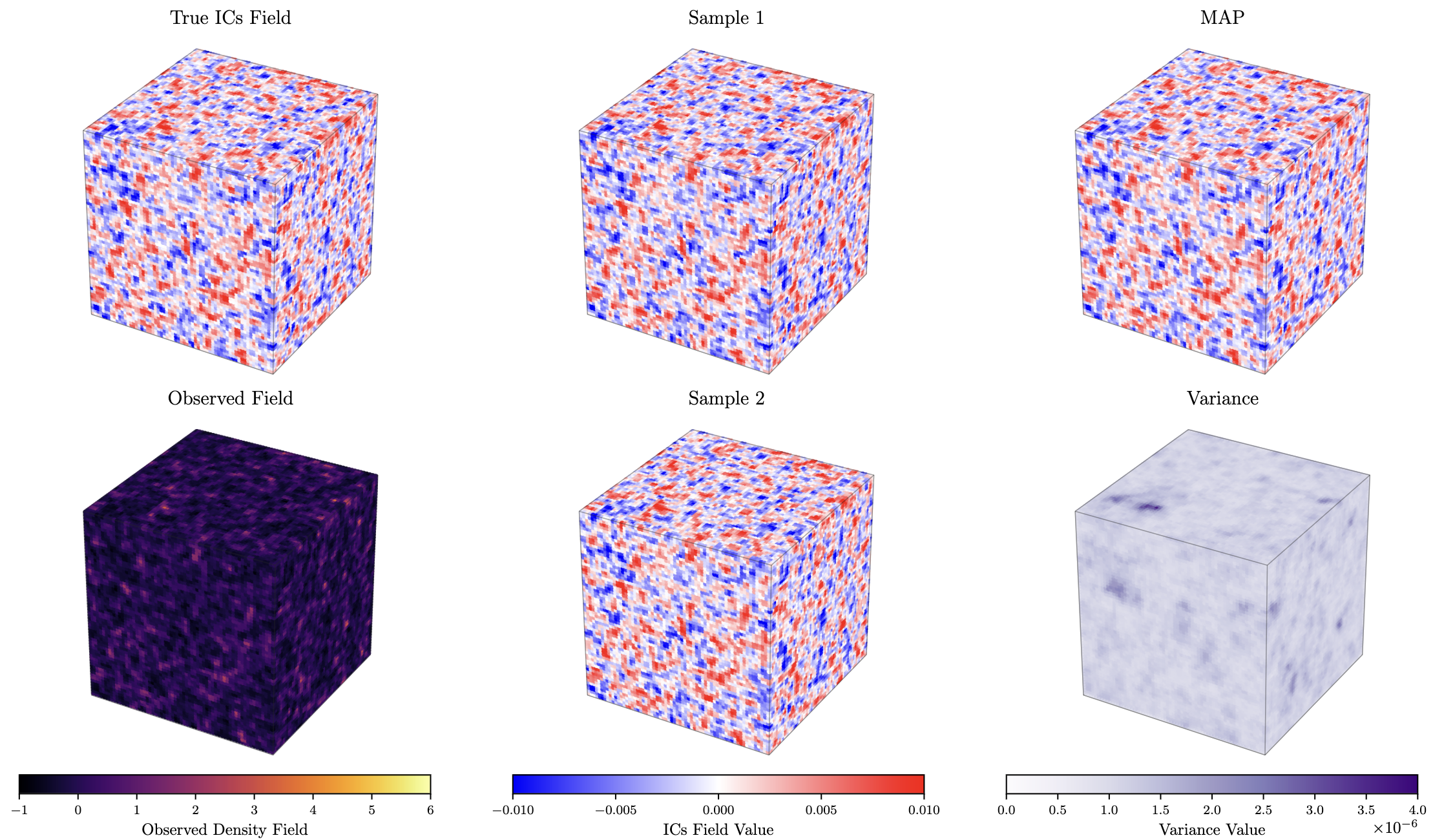
Training and sampling based on batched conjugate gradient
Training: 1.5 hrs on 1 GPU (NVIDIA A100 40GB)
Volume: \(V = (1\,\text{Gpc}/h)^3\), \(N_\mathrm{grid} = 64^3\)
\(10^3\) posterior samples in < 10 seconds

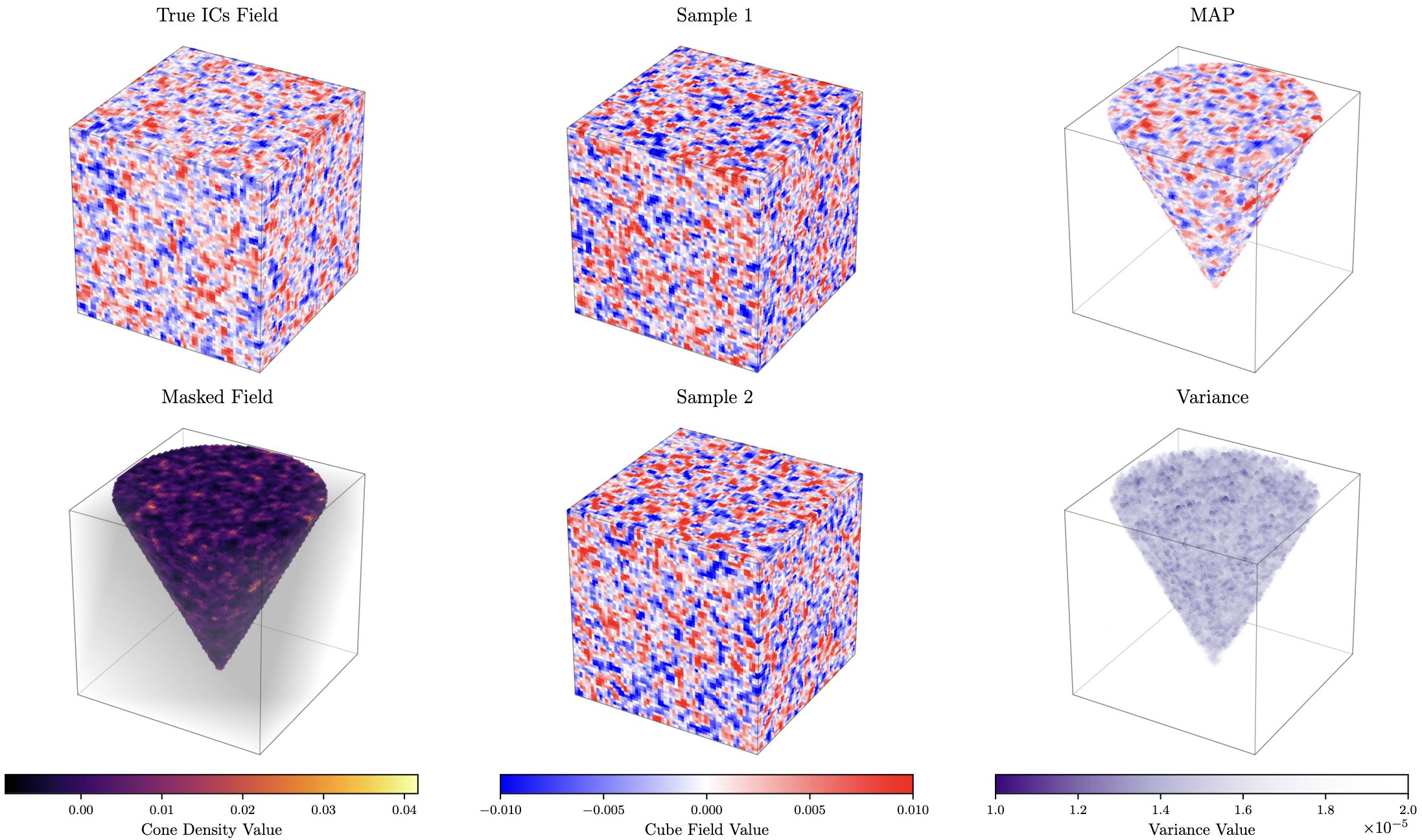
Training and sampling based on batched conjugate gradient
Training: 6 hrs on 1 GPU (NVIDIA A100 40GB)
Volume: \(V = (1\,\text{Gpc}/h)^3\), \(N_\mathrm{grid} = 64^3\)
\(10^3\) posterior samples in < 10 seconds

Diagnostics & verification

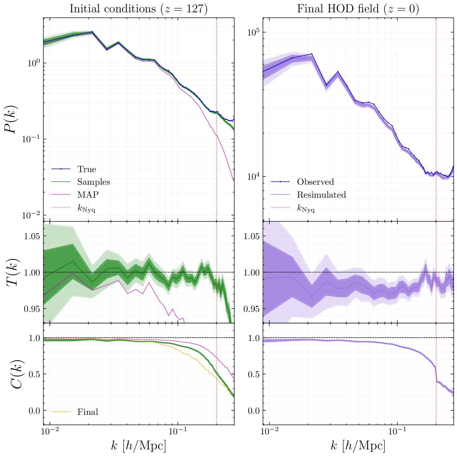
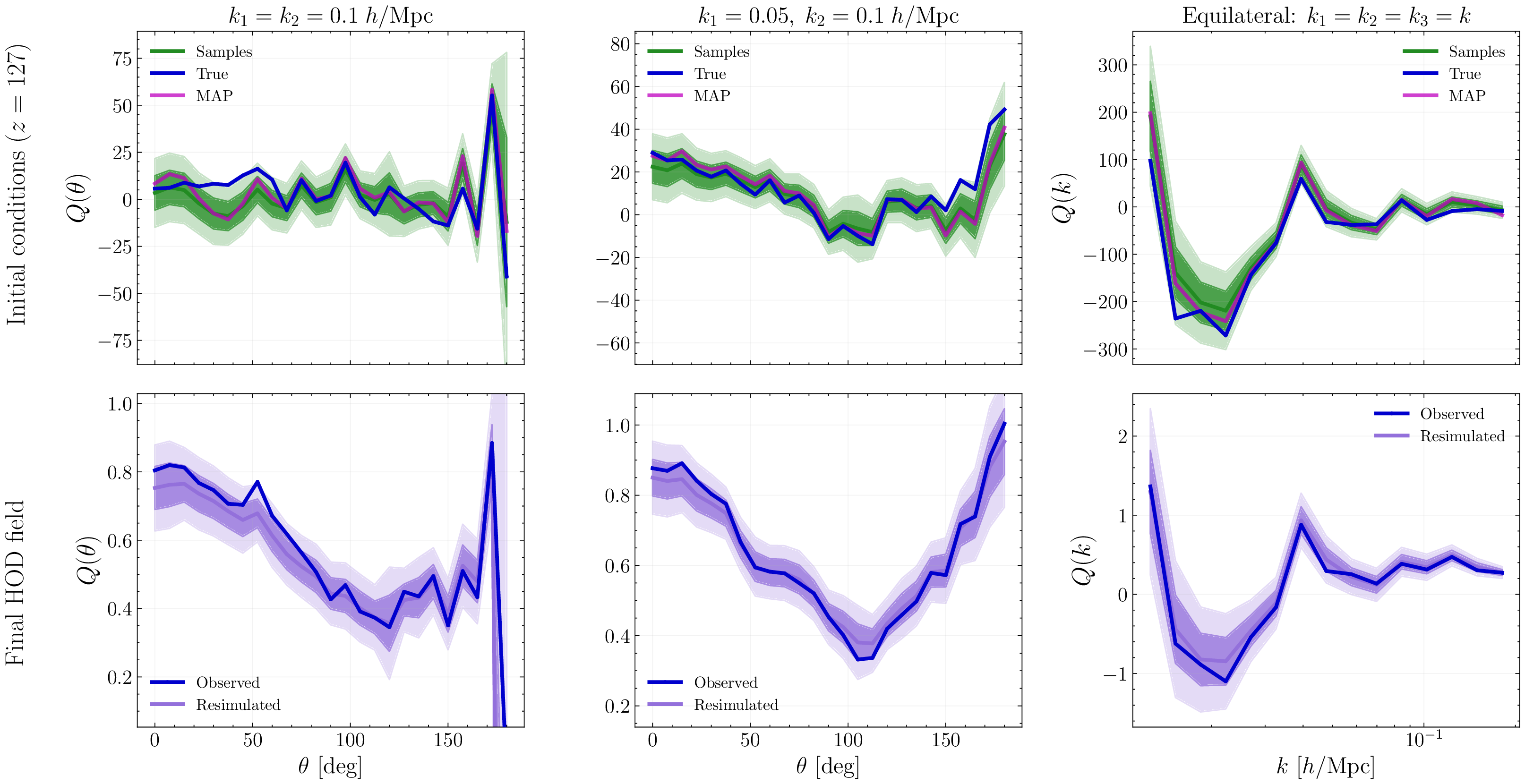
Summary statistics comparison: 1-point functions, power spectra, bispectra, Minkowski functionals, etc
Posterior predictive checks
Coverage tests

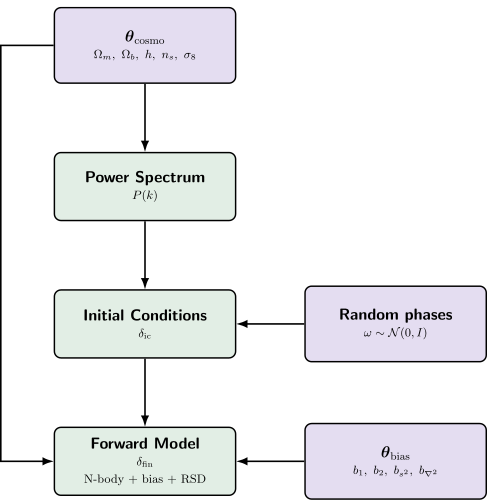
Forward model for adaptive case

A particle-mesh simulation evolves particles from the Lagrangian grid to Eulerian positions.
Each particle gets a tracer bias weight from the linear IC field: \(w(q) = 1 + b_1\,\delta(q) + b_2\,[\delta^2(q)-\langle\delta^2\rangle] + b_{s^2}\,[s^2(q)-\langle s^2\rangle] + b_{\nabla^2}\,\nabla^2\delta(q)\).
Bias-weighted particles are scattered and RSD-displaced to the mesh to form \(1 + \delta_{\mathrm{biased}}(x) = [\sum_q w(q)\,W(x-X(q))]/\langle\sum_q w(q)\,W(x-X(q))\rangle\).

List+, 2510.05206

Adaptive FLI

Use a tempered proposal \(\tilde p(\mathbf{z}) \propto p(\mathbf{x}_{\mathrm{obs}}\mid \mathbf{z})^{\gamma} p(\mathbf{z})\) to focus simulations on the region relevant for \(\mathbf{x}_{\mathrm{obs}}\).
Train on targeted pairs \(\mathbf{z} \sim \tilde p(\mathbf{z})\) and \(\mathbf{x} \sim p(\mathbf{x}\mid \mathbf{z})\).
The network learns \(q(\mathbf{z}\mid \mathbf{x})\) under this adapted proposal, so it is not the final posterior.
Recover \(p(\mathbf{z}\mid \mathbf{x}_{\mathrm{obs}})\) with an analytic correction involving \(q(\mathbf{z}\mid \mathbf{x}_{\mathrm{obs}})\), the original prior, and \(\gamma\).
For Gaussian NPE, this correction is available in closed form in precision space.

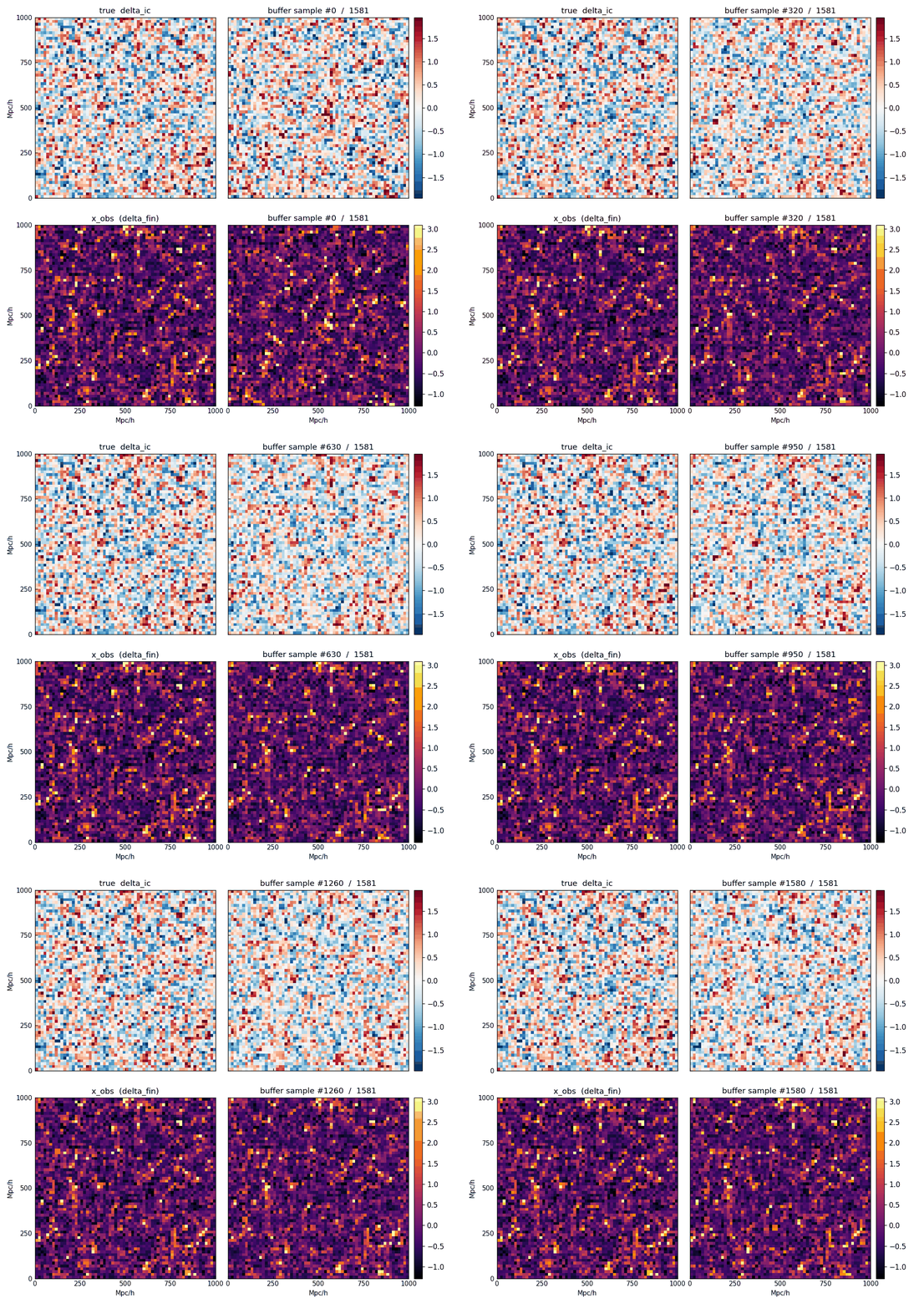
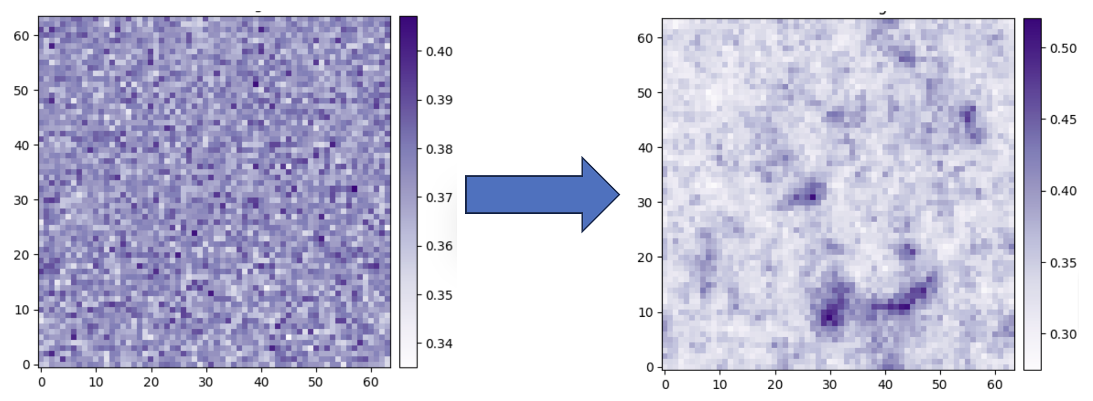
Adaptive training allows us to simplify the network architecture significantly, or remove some components entirely.
For example: U-Net \(\rightarrow\) trainable buffer

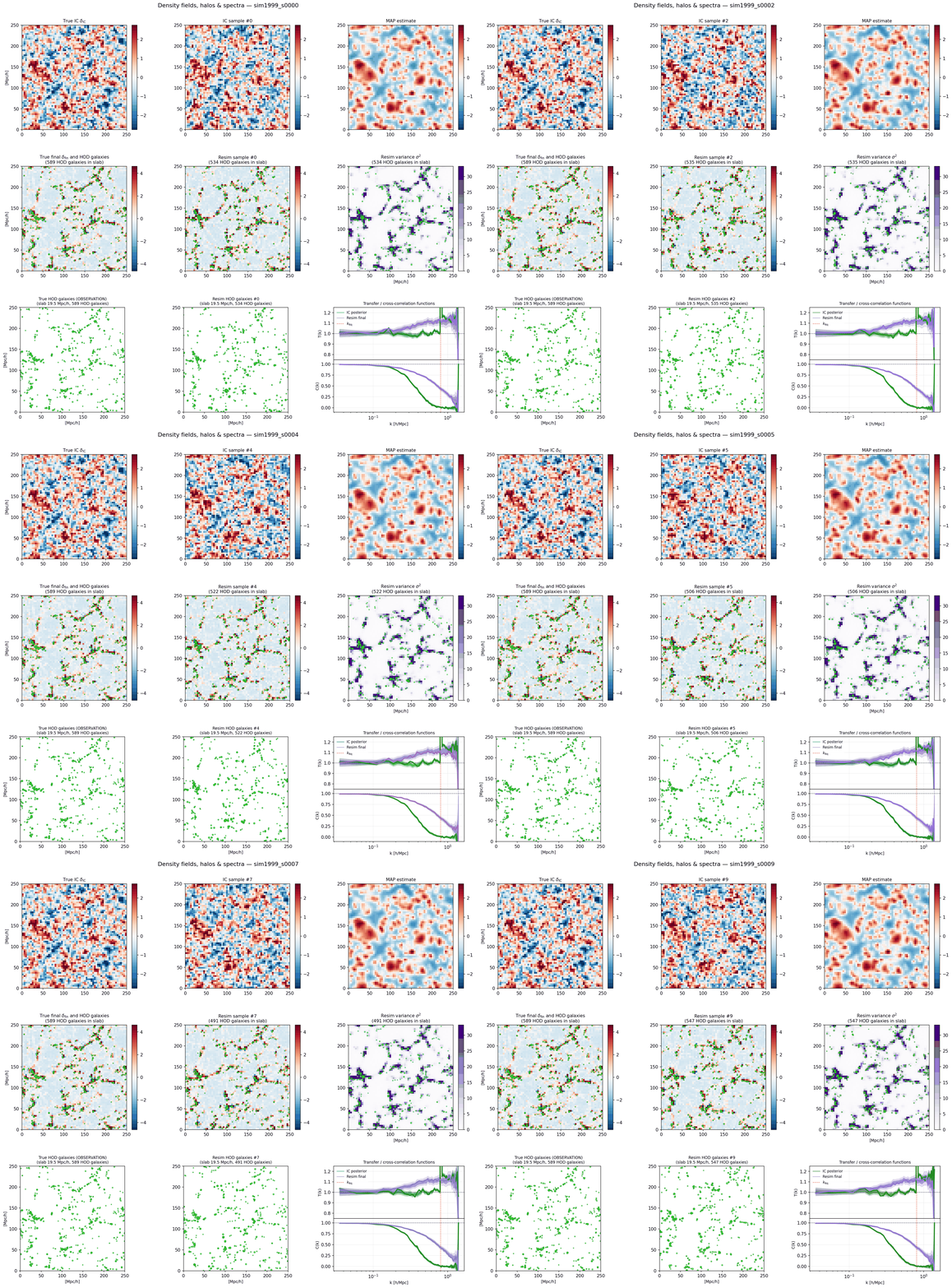
Variance of samples

Joint field + parameters inference

\(p(\boldsymbol{\delta}_{\mathrm{ICs}}, \boldsymbol{\theta}\mid\boldsymbol{\delta}_{\mathrm{obs}}) = p(\boldsymbol{\delta}_{\mathrm{ICs}}\mid\boldsymbol{\delta}_{\mathrm{obs}})\,p(\boldsymbol{\theta}\mid\boldsymbol{\delta}_{\mathrm{ICs}}, \boldsymbol{\delta}_{\mathrm{obs}})\)

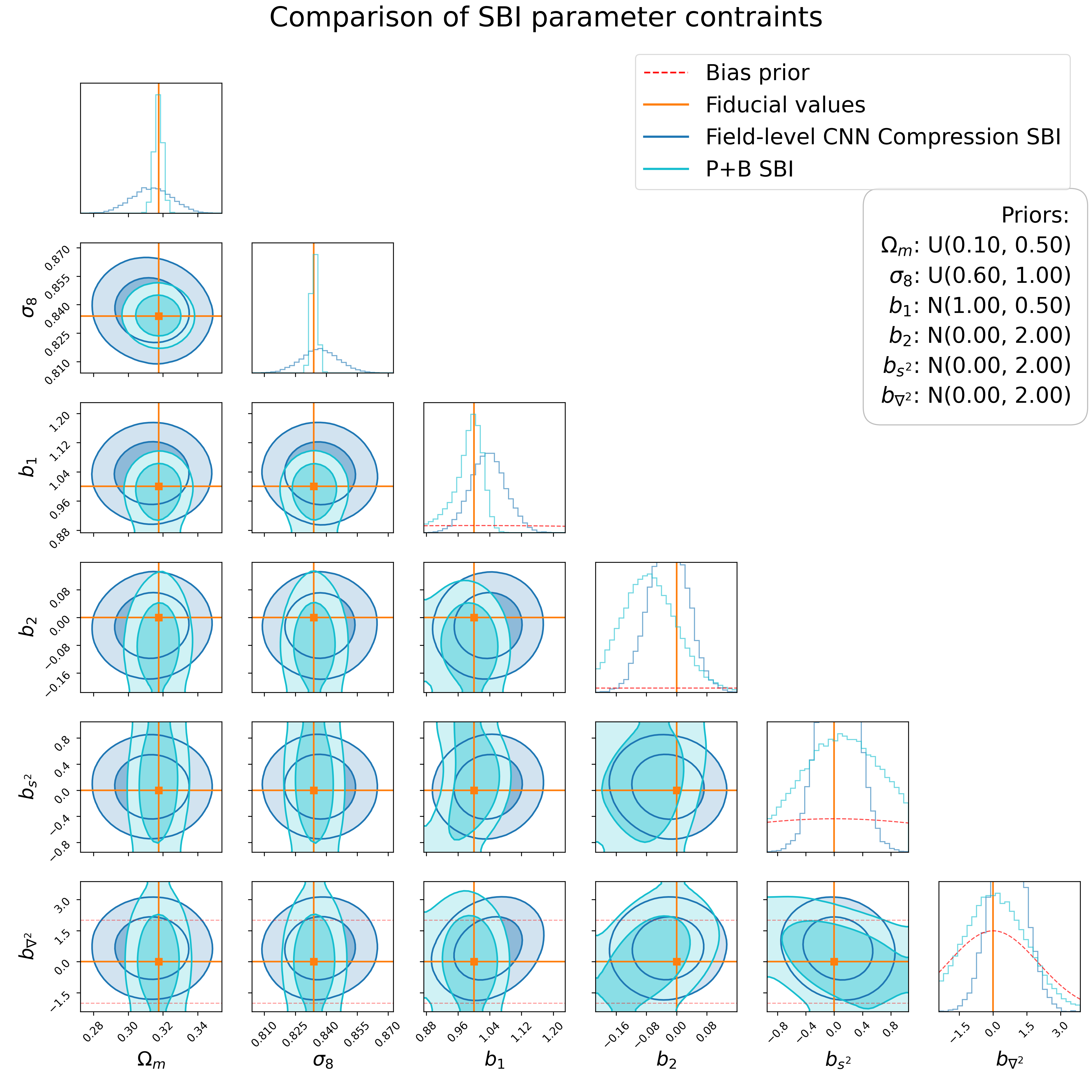
Adaptive SBI allows joint training of the two parts of the posterior
SBI allows to train optimal summaries by compressing fields
Inferring and compressing IC field gives better summaries

PRELIMINARY

Fields from point cloud data

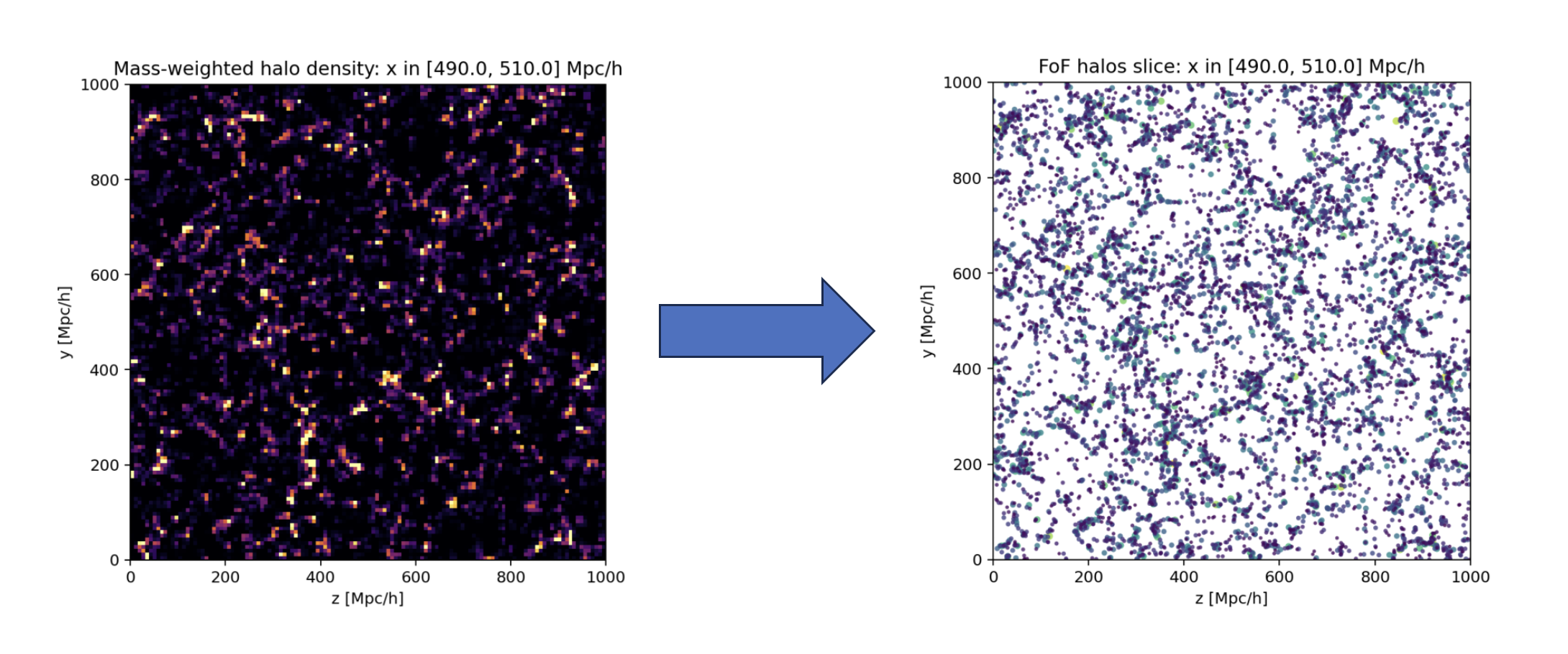
GNN architecture: Kvasiuk+ 2411.02496